Stata Fundamentals 1: Importing, inspecting and summarizing data
What is Stata?
Stata is a general purpose statistical analysis software, similar to SPSS. You can use it to preprocess, analyse and visualise data.
It is mostly used in research and particularly in the fields of economics, political science, and the social sciences in general.
In Stata you can either use the menus from the graphical user interface or write commands yourself. Most Stata users write commands and do not use the user interface. There are many advantages to learning commands. A script can be shared, edited by colleagues and collaborators and made available with publications. By using scripts for your research, you promote transparency and reproducibility. Since writing commands has many advantages and the majority of Stata users write scripts, we will also teach you how to write commands in this workshop series.
More information on how the session is run
What to do when getting stuck:- Ask the trainer if you struggle to find a solution.
- Use the help command. To get help with a specific command type help "command name"
- Search online. The statalist.org forum is usually the most useful resource.
- change the working directory
- import stata and csv documents
- print an overview of the variables in a dataset
- print a dataset and subsets of the data
- create a summary of continuous variables
Access to Datasets
Please use this link to get access to the datasets that you will be using in the exercises
Changing the working directory
When loading a dataset, Stata will always look for the file in the working directory, unless you specify the whole path to the file.
Although you can always specify the whole path to open a file that is not located in the working directory, it makes sense, to change the working directory to where your datasets are located at the beginning of your analysis. This will make it easier to load and switch between different datasets, since you only have to specify the file name and not the whole path to load a dataset.
Printing the current working directory
The working directory is displayed on the bottom of the main Stata window, just below the Command field.
You can also use the pwd command to print the working directory.
. pwd
/Users/michaelwiemers
Changing the working directory
You can change the working directory by using the cd command as below. Notice that the path has to be put in quotations.
. cd "/Users/michaelwiemers/OneDrive - London School of Economics/DSL/datasets/"
/Users/michaelwiemers/OneDrive - London School of Economics/DSL/datasets
Exercise: Changing the working directory
- Print the current working directory.
- Change the working directory to where the datasets lfs2017.dta, gapminder.csv and MCS_testscores.dta are located on your computer.
- Print the working directory again to verify that it has been changed.
Loading data into Stata
In this section you will learn how to import Stata datasets (.dta) and flat files, i.e. comma or tab separated value files (.csv or .tsv).
loading a .dta file (Stata dataset)
Now that Stata knows where your datasets are located, we can load a dataset without having to specify the whole path. We can simply refer to the file name.
We are going to load the lfs2017.dta file. This dataset contains data from the labour force survey from 2017. This dataset contains data on a persons age, sex, income, highest qualification and more.
We can load a .dta file, with the use command.
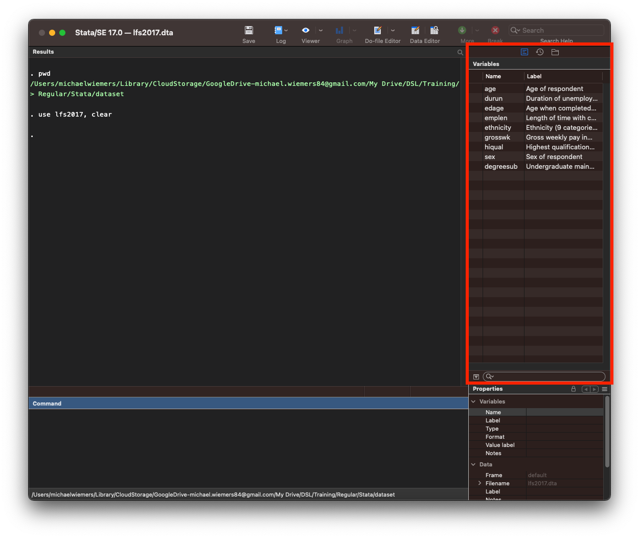
. use lfs2017
You can see that the variables pane on the right now lists all variables in the lfs2017 dataset.
Loading a public dataset from stata-press.com
There are a number of datasets in stata format available from the stata-press.com website. You can use this link for a list of all available datasets (unfortunately, without description):
https://www.stata-press.com/data/r15/u.html
To load the auto dataset from the stata website, we use the webuse command followed by the name of the dataset.
. webuse auto
(1978 Automobile Data)
Loading a csv file
We can use the import delimited command to import a csv file. In the example below we are importing the data stored in the gapminder.csv file, which is from the gapminder.org website, and lists unemployment, life expectancy and gdp per capita, for a sample of countries from across the world.
As you can see below, this commad returns an error. This is because we already have a dataset loaded in Stata and the error warns us that by loading the new dataset, unsaved changes to the currently loaded dataset might be lost.
. import delimited "gapminder.csv"
no; data in memory would be lost
r(4);
We have to first remove the currently loaded dataset with the clear command.
. clear

. import delimited "gapminder.csv"
(15 vars, 427 obs)
Alternatively, we can add clear as an option to the import delimited command or any other command to import data.
. import delimited "gapminder.csv", clear
(15 vars, 427 obs)
Exercise: Loading data
- Load the lfs2017 dataset using the use command.
- Load the citytemp.dta dataset from the Stata website.
- Load the csv file gapminder.csv.
- Notice how you can see the variables in the variables pane change everytime you load a different dataset.
Inspecting a dataset
In this section, we will focus on a few commands to inspect a dataset.
We’re first going to re-open the lfs2017 dataset.
. use lfs2017, clear
Summary of a dataset
The describe command produces a summary of a dataset. It lists the total number of observations, variables and the size of the dataset. Apart from the variable name and the variable label, which are also displayed in the Variables pane in the top right in the main Stata window, it also lists the storage type, display format and the value label.
The storage type refers to how the values of a variable are stored in memory. Different storage types can hold different types of information, i.e. numerical or text, and can store information of different size.
The display format refers to how the information is displayed, that is, the number of digits and decimals and the alignment.
The value label refers to the text labels that are being associated to the numerical values in the dataset. The sex variable has the numerical values 1 and 2, but when looking at the data you will see the labels ‘Female’ and ‘Male’ displayed. This is because the values 1 and 2 have received the corresponding labels ‘Male’ and ‘Female’.
describe

Contains data from lfs2017.dta
  obs:        10,096
 vars:             9                          3 Aug 2020 17:50
 size:       100,960
------------------------------------------------------------------------------------------------------------------------
              storage   display    value
variable name   type    format     label      variable label
------------------------------------------------------------------------------------------------------------------------
age             byte    %8.0g      AGE        Age of respondent
durun           byte    %8.0g      DURUN      Duration of unemployment
edage           byte    %8.0g      EDAGE      Age when completed full time education
emplen          byte    %8.0g      EMPLEN     Length of time with current employer
ethnicity       byte    %8.0g      ETHUKEUL   Ethnicity (9 categories) UK level
grosswk         int     %8.0g      GRSSWK     Gross weekly pay in main job (Government scheme or employee)
hiqual          byte    %8.0g      HIQUL15D   Highest qualification (detailed grouping)
sex             byte    %8.0g      SEX        Sex of respondent
degreesub       byte    %8.0g      UNCOMBMA   Undergraduate main subject area
------------------------------------------------------------------------------------------------------------------------
Sorted by:
Viewing the data
To display the entire dataset, we use the browse command. This will open the data editor.
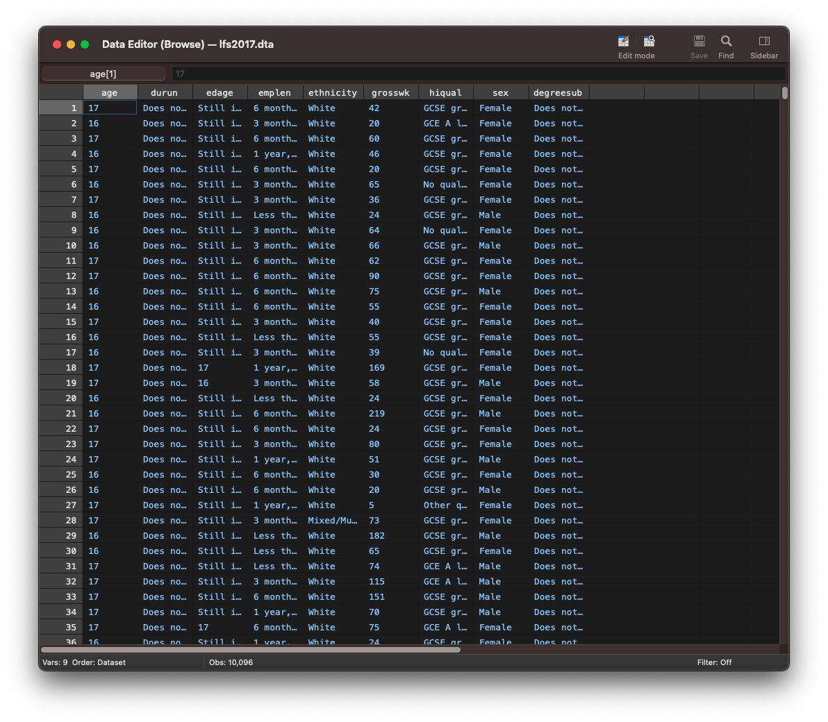
Printing only a subset of variables
To only display the observations for a specific variable, type browse followed by the variable name. Here, we are only printing the values for the age variable.
browse age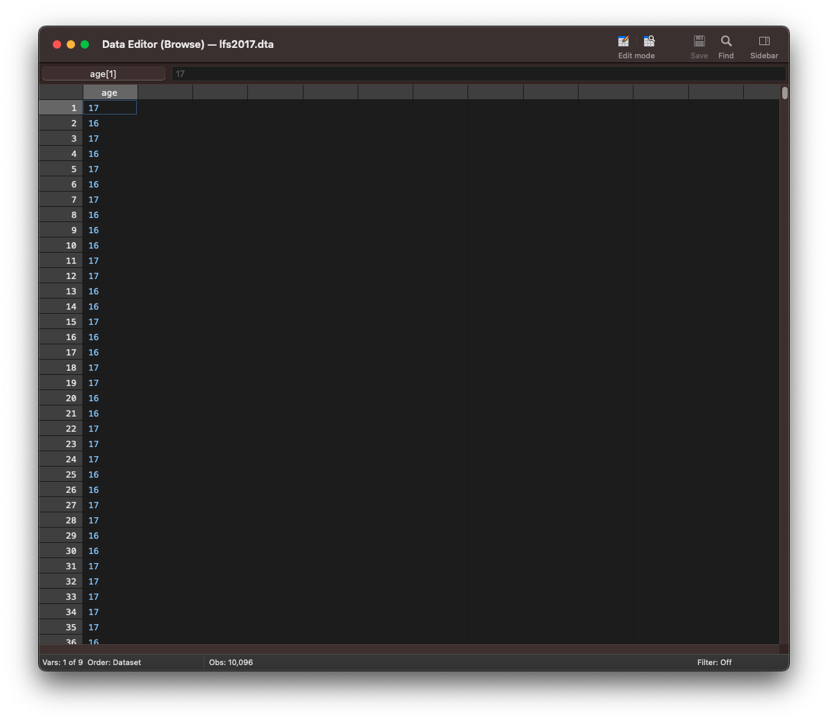
To display a subset of variables, type browse followed by the different variable names separated with a space.
browse age grosswk sex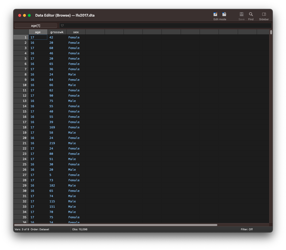
To display a range of variables type browse followed by the first variable, a hyphen and the last variable. The command browse grosswk - degreesub will print the observations for the variables starting from ethnicity till sex in the order as appearing in the dataset from left to right.
browse grosswk - degreesub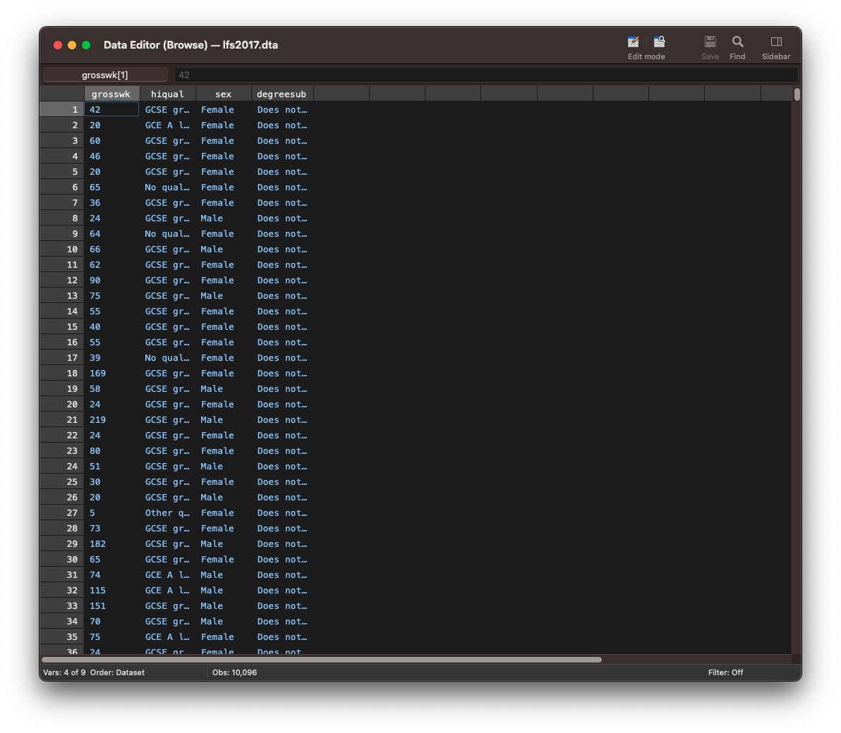
Exercise: Inspecting data
- Open the census5 dataset from the stata website, which has data from the 1980 US census
- Print an overview of the variables.
- View the census datasets.
- Print only the marriage and divorce variables.
Summary statistics
The summarize command gives you a number of descriptive statistics like the mean, standard deviation and the minimum and maximum value. We can abbreviate the summarize command as sum.
sum grosswk

    Variable |        Obs        Mean    Std. Dev.       Min        Max
-------------+---------------------------------------------------------
     grosswk |     10,096    521.7672    522.8757          5      23076
You can add the detail option to the command to also display the percentiles, variance, skewness and kurtosis.
sum grosswk, detail

     Gross weekly pay in main job (Government scheme or
                          employee)
-------------------------------------------------------------
      Percentiles      Smallest
 1%           34              5
 5%           90              5
10%          135              5       Obs              10,096
25%          250              5       Sum of Wgt.      10,096

50%          418                      Mean           521.7672
                        Largest       Std. Dev.      522.8757
75%          664          10250
90%          962          13846       Variance         273399
95%         1269          13846       Skewness       13.48147
99%         1923          23076       Kurtosis       448.2789
To summarize more than one continuous variable, add all variable names after sum.
sum grosswk sex

    Variable |        Obs        Mean    Std. Dev.       Min        Max
-------------+---------------------------------------------------------
     grosswk |     10,096    521.7672    522.8757          5      23076
         sex |     10,096    1.520503    .4996042          1          2
Customized summary statistics
The summarize command although useful to get a quick impression of a variable, doesn’t feature any options to select specific descriptives to be displayed in the output. The tabstat command allows such customisation of the statistics to be displayed.
tabstat age

    variable |      mean
-------------+----------
         age |  42.37223
------------------------
Exercise: Summary statistics
The MCS_testscore dataset contains data from the age 5 sweep from the Millenium Cohort Study, which examined the first year of primary schooling alongside childhood health, childcare, education, social and family circumstances.
- Open the MCS_testscore dataset.
- Use summarize to create a table with descriptive statistics for the variables pse to fsptotal.
- Use the tabstat command to create a table for the same variables Adjust your tabstat command to list the mean, standard deviation, standard error of the mean, min, max and the 25th and 75th percentile.
- Further adjust you command to ensure that the statistics are displayed in the columns.
Final task: Please give us your feedback!
Upon completing the survey, you will receive the link to the solution file, to check how your commands compares to the sample solution.
In order to adapt our training to your needs and provide the most valuable learning experience for you, we depend on your feedack.
We would be grateful if you could take 1 min before the end of the workshop to get your feedback!
Click here to open the survey!