Data cleaning in Stata - Variable and value labels
The data cleaning series is going to teach you the most fundamental commands and techniques to prepare data in Stata for statistical analysis.
The series is going to cover the following topics:
- Converting string to numerical
- Dealing with missings and duplicates
- Applying variable and value labels
- Reshaping and merging data
This session teaches you how to assign variable and value labels, which make your data and analysis output easier to read and interpret.
By the end of this session, you will know:
- about the importance of labelling variables and values
- how to apply variable labels
- how to create, apply and modify value labels
- how to turn a string variable into a numerical variable with corresponding value labels
- how to rename variable names with extracted variable labels
More information on how the session is run
How to work together:- Please turn on your microphone and webcam.
- One shares the screen and the other requests remote control.
- Take turns on who types for each exercise.
- Ask the trainer if you struggle to find a solution.
- Use the help command. To get help with a specific command type help "command name"
- Search online. The statalist.org forum is usually the most useful resource.
In this unit, you are going to learn about variable and value labels and the different commands available to create and apply labels.
Labels can be applied to either variables or the values of a variable. A variable label is a short description of the data that the variable contains. Value labels are labels that are displayed instead of the raw numerical values. You would apply value labels only to a categorical variable and not to a continuous variable, since for a categorical variable the numerical values represent a specific category and not a scale value.
Variable labels
A variable label is a short description of the type of data that the variable contains. As you might remember you can get a list of the label for each variable in your dataset with the describe command.
. webuse auto, clear
(1978 Automobile Data)
. describe

Contains data from http://www.stata-press.com/data/r15/auto.dta
obs:            74                          1978 Automobile Data
vars:            12                          13 Apr 2016 17:45
size:         3,182                          (_dta has notes)
----------------------------------------------------------------------------------------------------------------------------------------------------------------------------------------------------------------------------------------------------------
              storage   display    value
variable name   type    format     label      variable label
----------------------------------------------------------------------------------------------------------------------------------------------------------------------------------------------------------------------------------------------------------
make            str18   %-18s                 Make and Model
price           int     %8.0gc                Price
mpg             int     %8.0g                 Mileage (mpg)
rep78           int     %8.0g                 Repair Record 1978
headroom        float   %6.1f                 Headroom (in.)
trunk           int     %8.0g                 Trunk space (cu. ft.)
weight          int     %8.0gc                Weight (lbs.)
length          int     %8.0g                 Length (in.)
turn            int     %8.0g                 Turn Circle (ft.)
displacement    int     %8.0g                 Displacement (cu. in.)
gear_ratio      float   %6.2f                 Gear Ratio
foreign         byte    %8.0g      origin     Car type
----------------------------------------------------------------------------------------------------------------------------------------------------------------------------------------------------------------------------------------------------------
Sorted by: foreign
You can change the label of a variable with the label variable command. The label variable command takes as arguments the name of the variable and the variable label in double qoutes.
In the example below, we are changing the variable label of the variable price to Price (USD).
. label variable price "Price (USD)"
We can quickly check whether the label has been changed with describe
. describe  price

              storage   display    value
variable name   type    format     label      variable label
----------------------------------------------------------------------------------------------------------------------------------------------------------------------------------------------------------------------------------------------------------
price           int     %8.0gc                Price (USD)
Exercise 1: Variable labels
Run the code chunk to split the make variable into a variable for the brand and model.
. split make
. gen model = make2 + " " + make3
. rename make1 brand
. drop make*
- Create a variable label for the brand variable.
- Create a variable label for the model variable.
Value labels
In order to illustrate the concept of value labels, we are going to use a fictitious dataset on income data with variables on the respondents id, gender, employment sector and income.
We can enter data into Stata manually with the input command. After input we specify the names of the variables we want to enter, that is id, gender, sector and income and hit return. We can then enter the values for each observation in a separate line. In order to end the input of more observations, we use the end command.
. clear

. input id gender sector income
id     gender     sector     income
1. 1 1 4 30000
2. 2 2 2 50000
3. 3 1 3 10000
4. 4 2 2 40000
5. 5 1 1 120000
6. 6 2 4 20000
7. end
Value labels are labels that are displayed instead of the raw numerical values of a variable. Value labels are useful to add a label that describes the category that the raw numerical value represents.
The gender and sector variables are numerical variables where the numbers represent a specific category. In the gender column, 1 represents male and 2 represents female. Since the mapping is abritrary it makes sense to add labels to these numerical values so that the labels and not the raw numbers are displayed.
In the next two sections, you will learn how to add such labels to a categorical variable with numerical values.
Defining value labels
Creating value labels is a two step process, in which you first define the value label, that is, the mapping between raw values and labels and then apply that value label to a specific variable.
Below you can see how we can use the label define command to define the value label gender_lab which maps 1 to male and 2 to female.
Following label define, we first provide the name for the value label, that is, gender_lab. Subsequently, we define the mapping between each numerical value and its label. The first numerical value is 1, which is labelled male. The next numerical value is 2, which is labelled female.
. label define gender_lab 1 male 2 female
In order to list the mapping between values and labels in a value label, we can use the label list command. This command provides a quick way to verify that a label has been defined as intended.
. label list gender_lab
gender_lab:
1 male
2 female
Applying value labels
If we now list the data, we see that the label hasn’t yet been applied. We still only see the entered numbers in the gender column.
. list

   +-------------------------------+
   | id   gender   sector   income |
   |-------------------------------|
1. |  1        1        4    30000 |
2. |  2        2        2    50000 |
3. |  3        1        3    10000 |
4. |  4        2        2    40000 |
5. |  5        1        1   120000 |
   |-------------------------------|
6. |  6        2        4    20000 |
   +-------------------------------+
With the label define command we have only created the value label gender_lab, that is, the mapping of numerical values and labels (1 = male, 2 = female).
In order to apply the value label gender_lab to the variable gender, we can use the label value command. The label value command takes as first argument the name of the variable (gender) and as second argument the name of the value label (gender_lab)that should be applied to that variable.
. label value gender gender_lab
If we now use list the dataset, we can see that the gender variable no longer lists the numbers 1 and 2 but the labels male and female.
. list

   +-------------------------------+
   | id   gender   sector   income |
   |-------------------------------|
1. |  1     male        4    30000 |
2. |  2   female        2    50000 |
3. |  3     male        3    10000 |
4. |  4   female        2    40000 |
5. |  5     male        1   120000 |
   |-------------------------------|
6. |  6   female        4    20000 |
   +-------------------------------+
The labels male and female, however, have not replaced the raw numerical values 1 and 2. They are simply displayed instead of the raw numerical values. We can use the nolab option to display the numerical values instead.
. list, nolab

   +-------------------------------+
   | id   gender   sector   income |
   |-------------------------------|
1. |  1        1        4    30000 |
2. |  2        2        2    50000 |
3. |  3        1        3    10000 |
4. |  4        2        2    40000 |
5. |  5        1        1   120000 |
   |-------------------------------|
6. |  6        2        4    20000 |
   +-------------------------------+
To quickly check which value label has been applied to a variable, we can use codebook. In the second row it says label: gender_lab, which means that the value label gender_lab has been applied to the gender variable.
. codebook gender

----------------------------------------------------------------------------------------------------------------------------------------------------------------------------------------------------------------------------------------------------------
gender                                                                                                                                                                                                                                         (unlabeled)
----------------------------------------------------------------------------------------------------------------------------------------------------------------------------------------------------------------------------------------------------------

       type:  numeric (float)
      label:  gender_lab

      range:  [1,2]                        units:  1
unique values:  2                        missing .:  0/6

tabulation:  Freq.   Numeric  Label
              3         1  male
              3         2  female
Why using value labels for categorical data?
You might wonder why we would add value labels to a categorical variable instead of simply replacing the numerical values with string values?
Having a numerical variable makes it easier to use it for certain types of analyses. For instance, a linear regression analysis will not accept a string variable. An ordinal variable, that is, a variable whose categories have an inherent order, can be analysed with a linear regression, but only if in numerical format with labels/categories associated with each number.
Exercise 2: Value labels
- Enter the data with the below input command.
- Define the value label sector_lab for the sector variable, where the mapping
between the values and labels is:
- 1 - technology
- 2 - media
- 3 - energy
- 4 - transport
- List the number-value mappings of the sector_lab value label.
- Apply the value label to the sector variable.
- Print the dataset in the results pane to check that the value labels have been applied correctly.
clear all

input id gender sector income
1 1 4 30000
2 2 2 50000
3 1 3 10000
4 2 2 40000
5 1 1 120000
6 2 4 20000
end
Modifying value labels
Below we are adding another observation with the input command to our existing dataset.
. input

id     gender     sector     income
7. 7 3 3 35000
8. end
If we now print the dataset in the results pane, we notice that for the last observation no label is used for the value of the gender variable in the last row. That is because we didn’t add a label for the value 3, which codes for trans-female, when we defined the value label gender_lab.
. list

   +-------------------------------+
   | id   gender   sector   income |
   |-------------------------------|
1. |  1     male        4    30000 |
2. |  2   female        2    50000 |
3. |  3     male        3    10000 |
4. |  4   female        2    40000 |
5. |  5     male        1   120000 |
   |-------------------------------|
6. |  6   female        4    20000 |
7. |  7        3        3    35000 |
   +-------------------------------+
To add the mapping 3 trans_female to the existing value label gender_lab, we can use the label define command with the modify option.
This works very similar to when we defined the value label initially. After label define, we first specify the value label that we want to modify, that is, gender_lab. Next, we pass the numerical value and the corresponding label, that is, 3 trans_female, which we want to add to the existing value label. Finally, we add the option modify so that Stata knows we want to modify the existing value label gender_lab, instead of creating a new value label.
. label define gender_lab 3 trans_female, modify
As you can see, the changes are immediate, since the value label is already applied to the variable gender.
. list

   +-------------------------------------+
   | id         gender   sector   income |
   |-------------------------------------|
1. |  1           male        4    30000 |
2. |  2         female        2    50000 |
3. |  3           male        3    10000 |
4. |  4         female        2    40000 |
5. |  5           male        1   120000 |
   |-------------------------------------|
6. |  6         female        4    20000 |
7. |  7   trans_female        3    35000 |
   +-------------------------------------+
Exercise 3: Modfying value labels
- Modify the value label by changing the last mapping to 4 - transportation.
- Verify that the new pairing has been applied.
Using string values as value labels for a new numerical variable
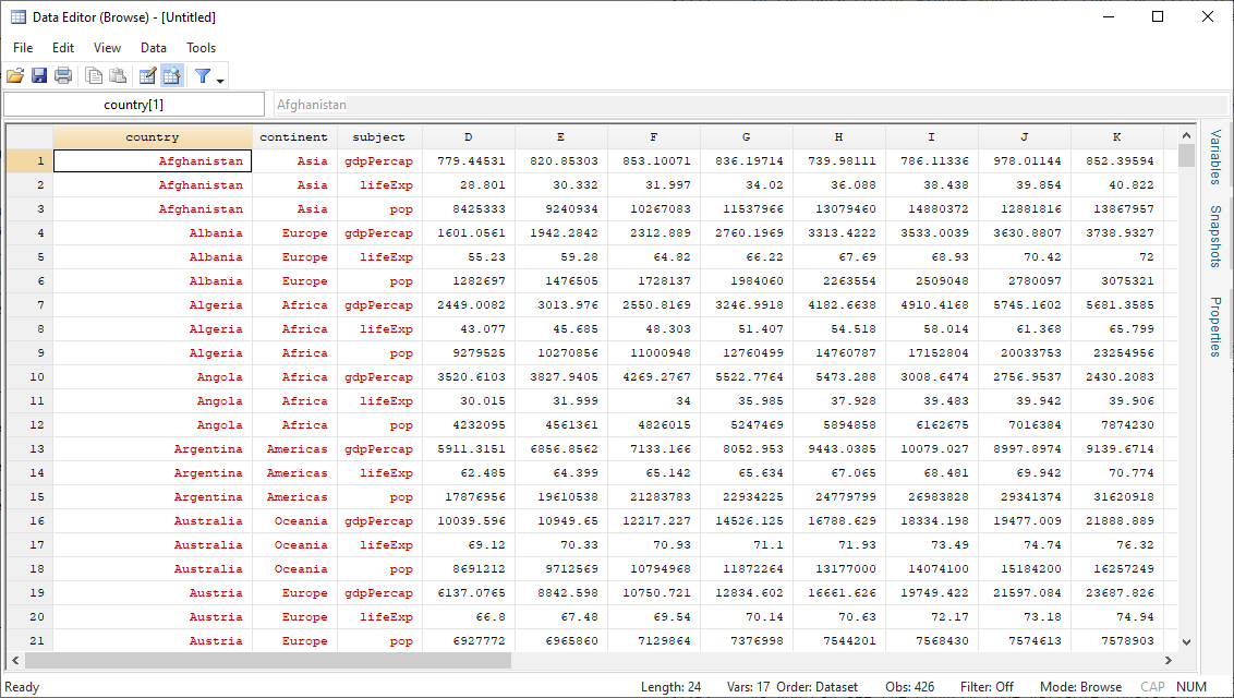
In this section we will continue to work with the gapminder and weo_data datasets. You are going to explore how you can create a numerical variable from an existing string variable and then apply the string values as labels to the numerical values.
In the data editor window you can see that the first few categorical variables in the gapminder dataset have been imported as string variables.
. import excel using "https://raw.githubusercontent.com/mwiemers/datasets/main/gapminder_dirty_labels.xlsx", ///
> firstrow clear

. browse
You can use the encode command in combination with the gen function to create a numerical variable country_code that uses the country names from the country variable as labels. The mapping of numbers to labels will be based on the alphabetical order of the string values.
Following encode you specify the name of the original string variable and with the gen option you can determine the name of the new numerical variable. The values from the string variable will be applied as labels to the values of the newly created numerical variable.
. encode country, gen(country_code)
As a final step we can delete the country variable. Rename the country_code variable to country and move it to first position with the order command.
. drop country

. rename country_code country

. order country
Exercise 4: String to numeric
- Load the weo_data_dirty_labels.xlsx dataset using the url “https://raw.githubusercontent.com/mwiemers/datasets/main/weo_data_dirty_labels.xlsx”. Make sure to import the variable names from the first row.
- Create a numerical version of the Country variable under the name Country_code.
- Remove the original Country variable and rename the Country_code variable to Country.
- Move the Country variable to the first position in the dataset with the order command.
Replace variable names with extracted variable labels
Stata doesn’t allow variable names to start with a number. The gapminder Excel file uses the date as a column name. When we import the Excel file with the firstrow option, Stata uses the column letters as the variable names and stores the actual column names, the dates (1952 - 2007), in the variable label, which we can inspect with the describe command.
. describe

Contains data
obs:           426
vars:            15
size:        49,842
----------------------------------------------------------------------------------------------------------------------------------------------------------------------------------------------------------------------------------------------------------
              storage   display    value
variable name   type    format     label      variable label
----------------------------------------------------------------------------------------------------------------------------------------------------------------------------------------------------------------------------------------------------------
country         long    %24.0g     country_code country
continent       str8    %9s                   continent
subject         str9    %9s                   subject
D               double  %10.0g                1952
E               double  %10.0g                1957
F               double  %10.0g                1962
G               double  %10.0g                1967
H               double  %10.0g                1972
I               double  %10.0g                1977
J               double  %10.0g                1982
K               double  %10.0g                1987
L               double  %10.0g                1992
M               double  %10.0g                1997
N               double  %10.0g                2002
O               double  %10.0g                2007
----------------------------------------------------------------------------------------------------------------------------------------------------------------------------------------------------------------------------------------------------------
Sorted by:
Note: Dataset has changed since last saved.
We can replace variables names with the rename command. Let us replace the variable name D with y1952. We can verify that the name has been changed by calling the describe command again.
. rename D y1952

. describe

Contains data
obs:           426
vars:            15
size:        49,842
----------------------------------------------------------------------------------------------------------------------------------------------------------------------------------------------------------------------------------------------------------
              storage   display    value
variable name   type    format     label      variable label
----------------------------------------------------------------------------------------------------------------------------------------------------------------------------------------------------------------------------------------------------------
country         long    %24.0g     country_code country
continent       str8    %9s                   continent
subject         str9    %9s                   subject
y1952           double  %10.0g                1952
E               double  %10.0g                1957
F               double  %10.0g                1962
G               double  %10.0g                1967
H               double  %10.0g                1972
I               double  %10.0g                1977
J               double  %10.0g                1982
K               double  %10.0g                1987
L               double  %10.0g                1992
M               double  %10.0g                1997
N               double  %10.0g                2002
O               double  %10.0g                2007
----------------------------------------------------------------------------------------------------------------------------------------------------------------------------------------------------------------------------------------------------------
Sorted by:
Note: Dataset has changed since last saved.
We can also create a local macro to extract and store the variable label and then use that local macro to rename the variable. Here, we create the local macro year, which extracts the variable label from the E variable.
We can then use the display command to show its value.
. local year: variable label E

. display `year'
1957
Let us now use the year macro to rename the E variable. We put the letter y in front of the year value, since the variable name has to start with a letter.
. rename E y`year'

. describe

Contains data
obs:            426
vars:            15
size:        49,842
----------------------------------------------------------------------------------------------------------------------------------------------------------------------------------------------------------------------------------------------------------
              storage   display    value
variable name   type    format     label      variable label
----------------------------------------------------------------------------------------------------------------------------------------------------------------------------------------------------------------------------------------------------------
country         long    %24.0g     country_code country
continent       str8    %9s                   continent
subject         str9    %9s                   subject
y1952           double  %10.0g                1952
y1957           double  %10.0g                1957
F               double  %10.0g                1962
G               double  %10.0g                1967
H               double  %10.0g                1972
I               double  %10.0g                1977
J               double  %10.0g                1982
K               double  %10.0g                1987
L               double  %10.0g                1992
M               double  %10.0g                1997
N               double  %10.0g                2002
O               double  %10.0g                2007
----------------------------------------------------------------------------------------------------------------------------------------------------------------------------------------------------------------------------------------------------------
Sorted by:
Note: Dataset has changed since last saved.
Instead of doing this manually for all the reaiming variables, we can write a for loop that loops over the variables from< i>F - O.
Inside the loop, we extract the variable label from each variable. Just like above, we create a new local macro under the name year by extracting the variable label from the variable that is currently stored with the var macro.
We then rename the variable stored with the var macro and replace it with the y followed by the year that is stored with the year macro.
. foreach var of varlist F-O{
      local year: variable label `var'
      rename `var' y`year'
}
Let us check whether the renaming worked.
. describe

Contains data
obs:           426
vars:            15
size:        49,842
----------------------------------------------------------------------------------------------------------------------------------------------------------------------------------------------------------------------------------------------------------
              storage   display    value
variable name   type    format     label      variable label
----------------------------------------------------------------------------------------------------------------------------------------------------------------------------------------------------------------------------------------------------------
country         long    %24.0g     country_code country
continent       str8    %9s                   continent
subject         str9    %9s                   subject
y1952           double  %10.0g                1952
y1957           double  %10.0g                1957
y1962           double  %10.0g                1962
y1967           double  %10.0g                1967
y1972           double  %10.0g                1972
y1977           double  %10.0g                1977
y1982           double  %10.0g                1982
y1987           double  %10.0g                1987
y1992           double  %10.0g                1992
y1997           double  %10.0g                1997
y2002           double  %10.0g                2002
y2007           double  %10.0g                2007
----------------------------------------------------------------------------------------------------------------------------------------------------------------------------------------------------------------------------------------------------------
Sorted by:
Note: Dataset has changed since last saved.
Exercise 5: Renaming variables with extracted variable labels
- Rename the C variable to y1980 without extracting the variable label with a local macro
- Extract the year from the variable label using a local macro and then rename the D variable using the local macro.
- Use a foreach loop for he remaining variables E-AK. Use the local macro var_name for the variale name. Inside the foreach loop, first extract the variable label from each varible using a local macro named var_year. Then rename the variable using the var_name and var_year macros, so that the new variables always start with the letter y followed by the year.
Final task: Please give us your feedback!
Upon completing the survey, you will receive the link to the solution file, to check how your commands compares to the sample solution.
In order to adapt our training to your needs and provide the most valuable learning experience for you, we depend on your feedack.
We would be grateful if you could take 1 min before the end of the workshop to get your feedback!