Data cleaning in Stata - Missings and duplicates
The data cleaning series is going to teach you the most fundamental commands and techniques to prepare data in Stata for statistical analysis.
The series is going to cover the following topics:
- Converting string to numerical
- Dealing with missings and duplicates
- Applying variable and value labels
- Reshaping and merging data
This session teaches you how to correctly label missing values and duplicates so that Stata can identify them as such when running an analysis or generating plots.
By the end of this session you will know how to:
- Find and delete duplicates.
- Identify observations containing missing values.
- Correctly label missing values.
- Dealing with missing values.
More information on how the session is run
How to work together:- Please turn on your microphone and webcam.
- One shares the screen and the other requests remote control.
- Take turns on who types for each exercise.
- Ask the trainer if you struggle to find a solution.
- Use the help command. To get help with a specific command type help "command name"
- Search online. The statalist.org forum is usually the most useful resource.
Loading the gapminder dataset
We load the gapminder dataset. So far, we have converted string variables to numerical. In the process, we have also already labelled all non-numerical string values as missing when we ran the destring v*, replace force command.
Today, we will remove duplicates, labell missing values and impute the missing values.
. import excel using https://raw.githubusercontent.com/mwiemers/datasets/main/gapminder_dirty_missings.xlsx, firstrow clear
Find and delete duplicates
The duplicate commands can help us to identify duplicated observations in our data. You can check out help duplicates to get a full list of all available commands.
To get an overview of whether the dataset contains any duplicates at all, we can use duplicates report.
. duplicates report

Duplicates in terms of all variables

--------------------------------------
   copies | observations       surplus
----------+---------------------------
        1 |          420             0
        2 |           12             6
--------------------------------------
In order to view the duplicated observations, we have to create a variable that records how many duplicates an observation has with duplicates tag, gen(). The gen option determines the name of the new variable.
. duplicates tag, gen(duplicated_n)

Duplicates in terms of all variables

. browse if duplicated_n > 0
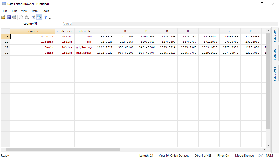
The duplicates drop command will drop all duplicated rows. We can verify that all duplicates have been dropped with duplicates report. The surplus column shows that there are no duplicates for the 426 observations in the dataset.
. duplicates drop

Duplicates in terms of all variables

(6 observations deleted)

. duplicates report

Duplicates in terms of all variables

--------------------------------------
   copies | observations       surplus
----------+---------------------------
        1 |          426             0
--------------------------------------
Exercise 1: Duplicates
weo_data.csv url:
https://raw.githubusercontent.com/mwiemers/datasets/main/weo_data_dirty_missings.xlsx
- Import the weo_data csv file using the above url. Make sure to import the variable names from row 1
- Print an overview of the number of duplicates in the data.
- Create a new variable that codes for whether an observation is duplicated.
- Print all observations that are duplicated.
- Remove all duplicated rows and print the overview of duplicates to verify that they have been removed.
Missing values
How does Stata represent missing values?
In Stata the . is the default symbol to represent missing numerical values. The extended missing values, .a, .b., c., …, .z can be used to represent specific types of numerical missings (don’t know, corrupted, etc.).
Empty quotes, "", are used to represent missing strings values.
Identify missings
When working with csv files, missings could be labelled as negative numbers in a variable that can only be positive, string values in a numerical variable or “n/a” in a categorical variable.
The first step in dealing with missing values, is therefore, to identify missing values. In the previous workshop on string variables, all numerical variables were imported as strings because of the comma and dollar symbol that they contained. When we converted them to numeric with the destring, replace force command any non-numerical values were directly converted into missing, that is, the . symbol.
A convenient way to get an overview of the number of missing values per variable, is the mdesc command, which is a user written command that is not part of Stata per default. You can install it with ssc install mdesc.
ssc install mdesc
Once installed, mdesc gives us the number of missing values and the percentage of missing values for each variable. As we can see, there is one value for the D - I variables that have been turned into a missing when we used the destring, force replace command in the previous workshop.
. mdesc

    Variable    |     Missing          Total     Percent Missing
----------------+-----------------------------------------------
        country |           0            426           0.00
      continent |           0            426           0.00
        subject |           0            426           0.00
              D |           1            426           0.23
              E |           1            426           0.23
              F |           1            426           0.23
              G |           1            426           0.23
              H |           1            426           0.23
              I |           1            426           0.23
              J |           0            426           0.00
              K |           0            426           0.00
              L |           0            426           0.00
              M |           0            426           0.00
              N |           0            426           0.00
              O |           0            426           0.00
   duplicated_n |           0            426           0.00
----------------+-----------------------------------------------
Those missing values that were labelled with a negative number, for instance -99, would not be converted to a . when using destring, force replace, since they are a legal numerical values. We can spot those values with the summarize command.
The variables D-H and L seem to use the value -99 to represent missing values.
. sum

    Variable |        Obs        Mean    Std. Dev.       Min        Max
-------------+---------------------------------------------------------
     country |          0
   continent |          0
     subject |          0
           D |        425     5602861    3.44e+07        -99   5.56e+08
           E |        425     6209378    3.88e+07        -99   6.37e+08
-------------+---------------------------------------------------------
           F |        425     6764566    4.14e+07        -99   6.66e+08
           G |        425     7571351    4.64e+07        -99   7.55e+08
           H |        425     8417479    5.25e+07        -99   8.62e+08
           I |        425     9249630    5.77e+07      31.22   9.43e+08
           J |        426    1.01e+07    6.22e+07     38.445   1.00e+09
-------------+---------------------------------------------------------
           K |        426    1.10e+07    6.79e+07     39.906   1.08e+09
           L |        426    1.20e+07    7.37e+07        -99   1.16e+09
           M |        426    1.29e+07    7.90e+07     36.087   1.23e+09
           N |        426    1.38e+07    8.35e+07     39.193   1.28e+09
           O |        426    1.47e+07    8.75e+07     39.613   1.32e+09
-------------+---------------------------------------------------------
duplicated_n |        426    .0140845     .117978          0          1
Correctly label missings
Once the data has been imported into Stata, we should use the . symbol to represent missing numerical values. Let us therefore replace the -99 values with the . symbol for the variables D - H and L using a foreach loop.
. foreach var of varlist D-H L{
	replace `var'=. if `var' == -99
}
(12 real changes made, 12 to missing)
(9 real changes made, 9 to missing)
(6 real changes made, 6 to missing)
(3 real changes made, 3 to missing)
(3 real changes made, 3 to missing)
(6 real changes made, 6 to missing)
We run the summarize command again to verify that the values have been changed to missings. The -99 values no longer show up in the Min column.
. sum

    Variable |        Obs        Mean    Std. Dev.       Min        Max
-------------+---------------------------------------------------------
     country |          0
   continent |          0
     subject |          0
           D |        413     5765659    3.49e+07     28.801   5.56e+08
           E |        416     6343717    3.92e+07     30.332   6.37e+08
-------------+---------------------------------------------------------
           F |        419     6861435    4.17e+07     31.997   6.66e+08
           G |        422     7625177    4.66e+07      34.02   7.55e+08
           H |        422     8477319    5.27e+07       35.4   8.62e+08
           I |        425     9249630    5.77e+07      31.22   9.43e+08
           J |        426    1.01e+07    6.22e+07     38.445   1.00e+09
-------------+---------------------------------------------------------
           K |        426    1.10e+07    6.79e+07     39.906   1.08e+09
           L |        420    1.21e+07    7.42e+07     23.599   1.16e+09
           M |        426    1.29e+07    7.90e+07     36.087   1.23e+09
           N |        426    1.38e+07    8.35e+07     39.193   1.28e+09
           O |        426    1.47e+07    8.75e+07     39.613   1.32e+09
-------------+---------------------------------------------------------
duplicated_n |        426    .0140845     .117978          0          1
If we run the mdesc command again, we notice that the data now also has
missing values for the D-H and L variables.
. mdesc

    Variable    |     Missing          Total     Percent Missing
----------------+-----------------------------------------------
        country |           0            426           0.00
      continent |           0            426           0.00
        subject |           0            426           0.00
              D |          13            426           3.05
              E |          10            426           2.35
              F |           7            426           1.64
              G |           4            426           0.94
              H |           4            426           0.94
              I |           1            426           0.23
              J |           0            426           0.00
              K |           0            426           0.00
              L |           6            426           1.41
              M |           0            426           0.00
              N |           0            426           0.00
              O |           0            426           0.00
   duplicated_n |           0            426           0.00
----------------+-----------------------------------------------
Exercise 2: Identify and label missings
- Install the mdesc command.
- Create an overview of the missings per variable.
- Use sum to identify any not-correctly represented missing values.
- Replace the values with the . symbol. Use a foreach loop for this.
- Use sum and mdesc commands to verify that the -99 values have been changed to missing.
Exploring missing values
Once all missing values have been correctly labelled, we might want to inspect observations with missing values more closely. We can generate a new variable with the number of missing values per observation with the rowmiss command.
. egen nmiss=rowmiss(*)
We have added a new variable nmiss to the dataset that codes for the number of missing values per row.
. browse in 1/10
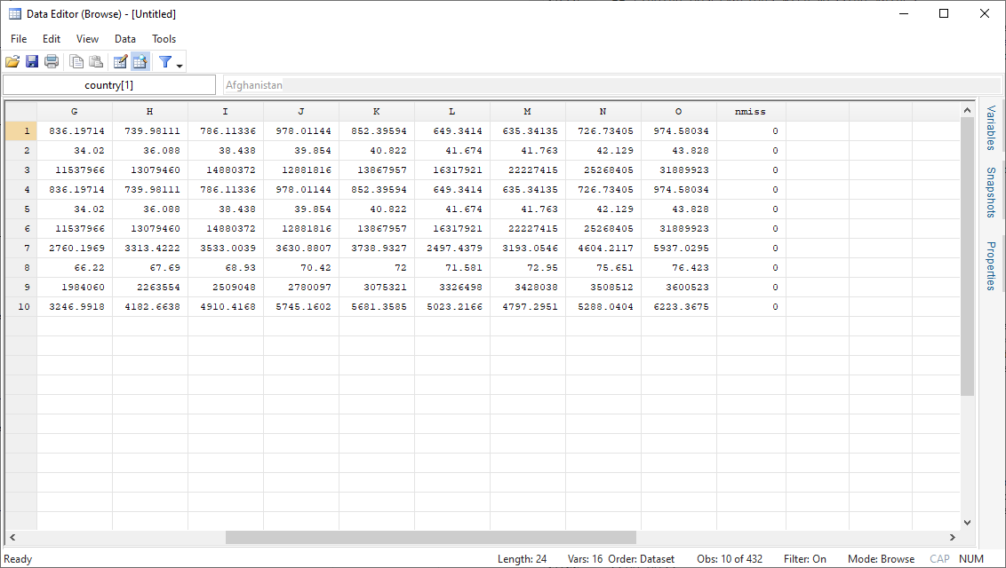
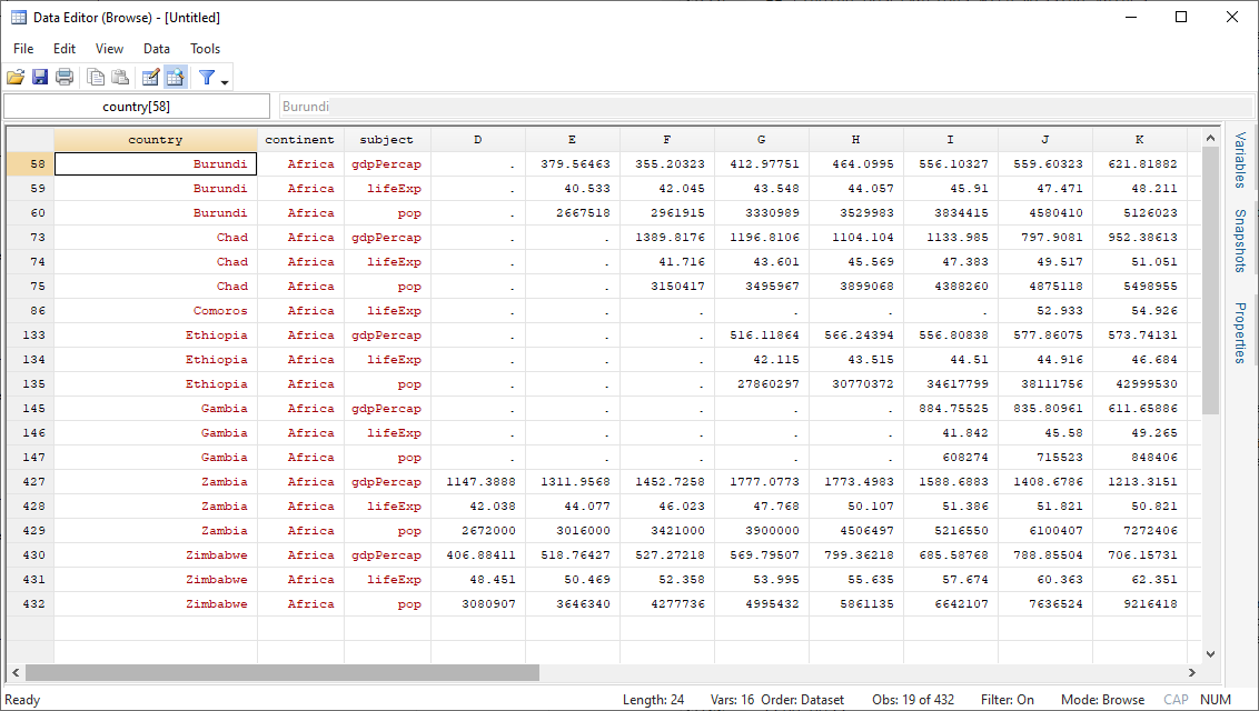
We can now have a look on the subset of the observations that includes missing values in the Data Editor. With the if qualifer if nmiss>0, we limit the output to those observations where nmiss has the value 1 or larger, that is, where there is at least 1 missing value.
. browse if nmiss>0
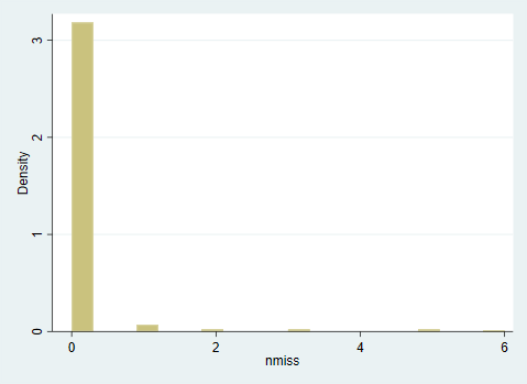
To get a sense of the distribution of missing values across observations, we can plot a histogram. This will help us to understand whether there are a lot of observations with a few missings or whether there are a few observations with a lot of missings.
. hist nmiss
(bin=20, start=0, width=.3)
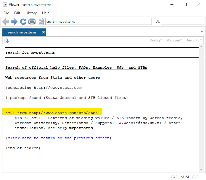
Another way we can look for specific patterns in the missings is by using the mvpatterns command. The mvpatterns command is not built-in into Stata and has to be installed first. In order to install it, we have to use the search command, which will open the viewer with any results related to the search term.
search mvpatterns
We click on the first link to open the mvpatterns page
We then click on the install link, which starts the installation.
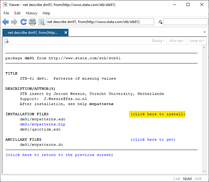
Once installed, we can now use the mvpatterns command, which returns a table with the number of missings for all variables with missing values and a second table that provides a list of all patterns of missings. The table indicates the pattern, that is, where inside the variables with missings the missing values occur (_pattern), the number of missings per pattern (_mv), and how often the pattern occurs (_freq).
The output helps us to quickly discover that a missing for variable D is the most frequent missing pattern. Patterns might be useful to better understand what causes missings in the data.
. mvpatterns
variables with no mv's: country continent subject J K M N O duplicated_n nmiss

Variable     | type     obs   mv   variable label
-------------+-----------------------------------
D            | double   413   13   1952
E            | double   416   10   1957
F            | double   419    7   1962
G            | double   422    4   1967
H            | double   422    4   1972
I            | double   425    1   1977
L            | double   420    6   1992
-------------------------------------------------

Patterns of missing values

  +------------------------+
  | _pattern   _mv   _freq |
  |------------------------|
  |  +++++++     0     407 |
  |  ++++++.     1       6 |
  |  .++++++     1       3 |
  |  ..+++++     2       3 |
  |  ...++++     3       3 |
  |------------------------|
  |  .....++     5       3 |
  |  ......+     6       1 |
  +------------------------+
Exercise 3: Exploring missing values
- Create a new variable for the number of missing values per row.
- Have a look at all observations with missing values in the Data Editor.
- Install the mvpatterns command.
- Print the pattern of missing values. What is the most common pattern?
Dealing with missing values
Dropping variables
If a substantial amount of the values for a specific variable is missing, you might consider to remove it from your dataset. This is usually only adviced if at least 60% of the values are missing and the variable itself doesn’t seem to play a significant role for your model.
We can drop a variable using the drop command. Since there are only 3 percent of the values missing for the D variable, it wouldn’t make sense to remove the variable.
drop D
Mean imputation
Imputing missing data is a complex topic that we cannot cover comprehensively in this workshop. A very basic approach to dealing with missings values is replacing them with the mean or median of the variable. In order to do that, we first have to use the summarize command, so that we can retrieve the mean of the D variable with `r(mean)’ in the replace command.
sum D
replace D=`r(mean)' if D==.
This is a common approach that is generally not advised, since it requires the values to be missing completely at random (MCAR). MCAR means, that neither the missing values itself nor other variables in the dataset can predict the missing values. This is rather strong assumption, that almost never is met. Missing values for an income variable, for instance, are likely to be extreme values, either very high or low incomes and are therefore predicting itself. Missing values might also be predicted based on another variable in the data. For instance, male respondents might be less likely to report income compared to women because of perceived social norms and stereotypes.
If the missigs are not MCAR, mean imputation will lead to biases in how the model parameters are estimated. Even if the MCAR assumption is met, mean imputation reduces the variance of the imputed variable and reduces the correlation with other variables in the data, which will impair your regression models.
Complete case analysis
Complete case analysis or listwise deletion is the technique of disregarding any non-complete cases for your statistical analyses. If your dependent or predictor variable have missing values, Stata will remove those cases from your data before running the analysis per default. Similar to mean imputation, this approach is only advided when data is missing MCAR, since it otherwise will induce biased parameter estimations. It also will lead to a loss of power, which might not be a problem depending on the size of your data.
Multiple imputation
There are more advanced techniques that have weaker assumptions about how the data are missing and will lead to less biased estimations. Multiple imputation (MI) is one of these techniques, that can be applied in Stata rather easily although you will have to consult the documentation to chose the most appropriate imputation method. MI does assume your data to be missing at random (MAR). Data is assumed to be MAR, when the variable itself does not predict its own missings, but other variables in the data do predict the missing values.
In basic terms, multiple imputation predicts missing values based on the available values in your data using a specific imputation method and creates a number of imputed datasets. All of the imputed versions of the data are then being analysed with the specific model to test your research hypothesis and the results are being pooled to provide a combined model.
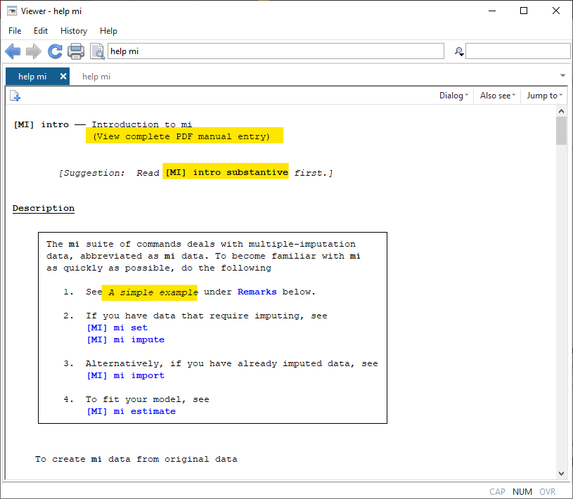
If you want to know more about MI in Stata, you can read this tutorial. The Stata documentation also provides very detailed description of it, which you can access with help mi command.
help mi
The main mi help page provides links to the manual, the comprehensive introduction, a simple example and links to the specific sub commands.
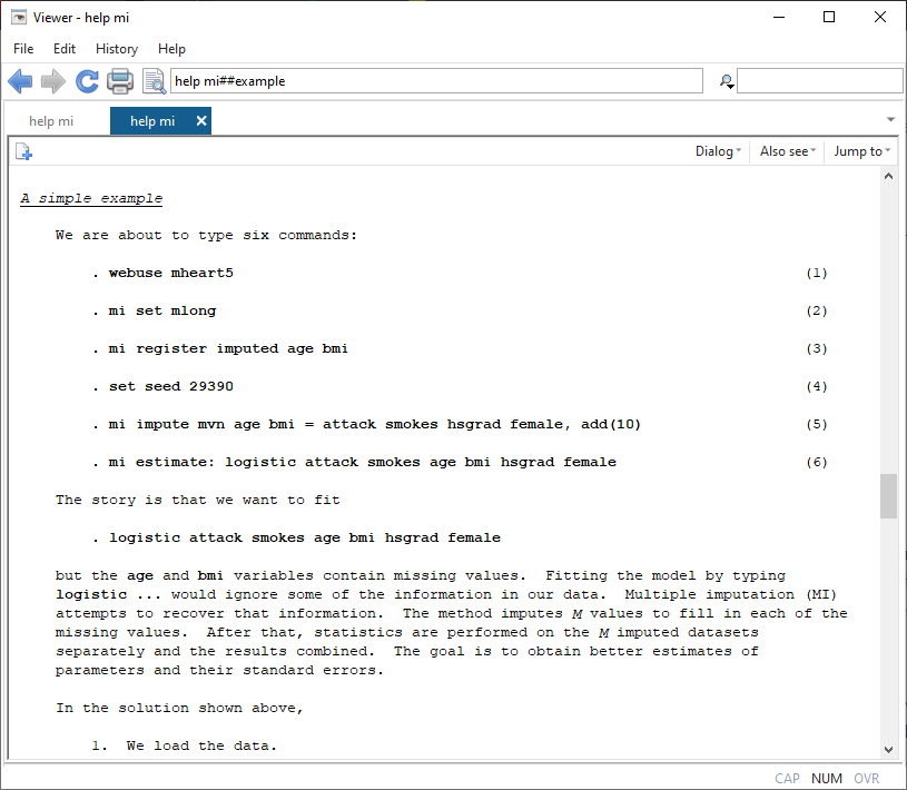
Below is a complete simple example of applying MI with Stata.
Final task: Please give us your feedback!
Upon completing the survey, you will receive the link to the solution file, to check how your commands compares to the sample solution.
In order to adapt our training to your needs and provide the most valuable learning experience for you, we depend on your feedack.
We would be grateful if you could take 1 min before the end of the workshop to get your feedback!