Data cleaning in Stata - Strings
The data cleaning series is going to teach you the most fundamental commands and techniques to prepare data in Stata for statistical analysis.
The series is going to cover the following topics:
- Converting string to numerical
- Dealing with missings and duplicates
- Applying variable and value labels
- Reshaping between long and wide format
- Merging multiple datasets
This sessions teaches you how to prepare string columns to a format that is suitable for data analysis and how to convert a string column with numerical values.
By the end of this session, you will know how to:
- Identify numerical values that have been imported as strings
- Modifying string values
- Convert strings to numerical
- Removing whitespace
- Splitting and combining string values
More information on how the session is run
How to work together in the Zoom sessions:- Plesase turn on your microphone and webcam.
- One shares the screen and the other requests remote control.
- Take turns on who types for each exercise.
- Ask the trainer if you struggle to find a solution.
- Use the help command. To get help with a specific command type help "command name"
- Search online. The statalist.org forum is usually the most useful resource.
Properties of clean data
What do we mean, when we talk about clean vs unclean data? Here are some of the key features of clean data:
- Numerical values are in a numerical format (integer or float)
- Missing values are clearly labelled as missing
- The data does not contain any duplicates
- Categorical columns are in numerical format using text labels
- Variables are meaningfully named and labelled
- Text and numerical variables have been inspected for corrupted values and cleaned
- The data should be in long format, where the levels of a repeated measurement are represented by a single variable and not spread out across several columns
The main reasons why data should be cleaned in a way outlined in the above list, is that it will prevent errors from commands that assume data to be in that particular format. For instance, Stata assumes data to be in long format for statistical analysis involving repeated measures and categorical variables to be using numerical values instead of strings. All of the above listed aspects of cleaning data will be addressed in the data cleaning workshop series.
Converting strings to numerical
Importing the gapminder.xlsx dataset
We import the gapminder.xlsx dataset with the import excel command. Since the data is coming from an url, we have to put using before the url. Since the first row contains the variable names, we use the firstrow option to set the values from the first row in the csv file as the variable names.
. import excel using https://github.com/mwiemers/datasets/raw/main/gapminder_dirty_strings.xlsx, firstrow clear
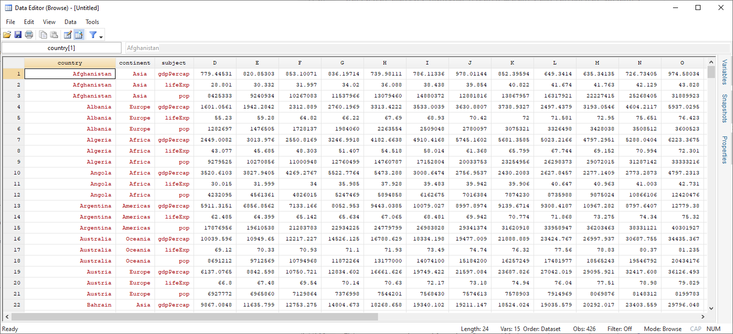
Let us have a quick look at the data.
The gapminder dataset contains data on GDP, population and life expectancy across the world. Each row represents values for a country. The actual values for the years 1952 to 2007 are in the D - O variables.
. br
Identifying numerical values in string format
In this unit you are going to learn how to convert variables that contain numerical data but have been imported into Stata as string, i.e. text variables, into a numerical format.
Sometimes numeric variables are displayed using a dot in csv files or a comma in Excel files to separate thousands, which makes large numbers easier to read. This can cause the problem that Stata will import them as strings, since for numerical variables there is no other symbol allowed apart from the dot as a decimal separator.
It is therefore a good habit to always inspect a dataset after having imported it to spot variables that need to be converted to a different format.
After having imported the gapminder dataset, we are going to inspect how the variables have been imported with describe.
. describe

Contains data
  obs:           432
vars:            15
size:        90,288
----------------------------------------------------------------------------------------------------------------------------------------------------------------------------------------------------------------------------------------------------------
              storage   display    value
variable name   type    format     label      variable label
----------------------------------------------------------------------------------------------------------------------------------------------------------------------------------------------------------------------------------------------------------
country         str24   %24s                  country
continent       str8    %9s                   continent
subject         str9    %9s                   subject
D               str13   %13s                  1952
E               str13   %13s                  1957
F               str13   %13s                  1962
G               str13   %13s                  1967
H               str13   %13s                  1972
I               str13   %13s                  1977
J               str15   %15s                  1982
K               str15   %15s                  1987
L               str15   %15s                  1992
M               str15   %15s                  1997
N               str15   %15s                  2002
O               str15   %15s                  2007
----------------------------------------------------------------------------------------------------------------------------------------------------------------------------------------------------------------------------------------------------------
Sorted by:
    Note: Dataset has changed since last saved.
All variables have been imported as string, which makes sense for the first three variables, which are categorical variables that contain text data. The remaining variables for the years from 1952 - 2007 however all contain numerical data.
We can get a quick overview of the data that is stored in the D-O variables with list.
The D-O variables use a comma to group the thousands as you can see in the third and fourth row.
. list D-O in 1/5

   +---------------------------------------------------------------------------------------------------------------------------------------------------------------------------------+
   |           D             E              F              G              H              I              J              K              L              M              N              O |
   |---------------------------------------------------------------------------------------------------------------------------------------------------------------------------------|
1. | 779.4453145   820.8530296      853.10071    836.1971382    739.9811058      786.11336    978.0114388    852.3959448    649.3413952     635.341351    726.7340548    974.5803384 |
2. |      28.801        30.332         31.997          34.02         36.088         38.438         39.854         40.822         41.674         41.763         42.129         43.828 |
3. | 8,425,333.0   9,240,934.0   10,267,083.0   11,537,966.0   13,079,460.0   14,880,372.0   12,881,816.0   13,867,957.0   16,317,921.0   22,227,415.0   25,268,405.0   31,889,923.0 |
4. | 779.4453145   820.8530296      853.10071    836.1971382    739.9811058      786.11336    978.0114388    852.3959448    649.3413952     635.341351    726.7340548    974.5803384 |
5. |      28.801        30.332         31.997          34.02         36.088         38.438         39.854         40.822         41.674         41.763         42.129         43.828 |
   +---------------------------------------------------------------------------------------------------------------------------------------------------------------------------------+
Removing illegal characters before converting
In order to convert a variable that is in string format to numeric, we first have to remove any illegal characters. We have identified the commas in the D-O variables in the previous step. We can remove the commas with the replace command in combination with the subinstr() function.
. replace D=subinstr(D,",", "", .)
(242 real changes made)
We use replace to make changes to the values in the variable D. In particular, we want to replace every comma with an empty string. In order to do so, we must ust the subinstr() function after the = sign.
The subinstr() function takes four arguments. The first is the variable we want to replace - D. The second argument is the value inside the variable, that we want to replace - the comma. The third argument is the value that we want to replace the comma with - an empty string. With the last argument you can specify how often you want to apply changing a comma to an empty string. It could be that there are only two commas in the variable that you want to replace. In that case you would enter a 2. By entering a . we instruct subinstr() to replace all occurences of the comma inside the values of the D variable with an empty string.
Below we replace the commas in all remaining variables with an empty string.
. replace D=subinstr(D,",", "", .)
(0 real changes made)

. replace E=subinstr(E,",", "", .)
(245 real changes made)

. replace F=subinstr(F,",", "", .)
(252 real changes made)

. replace G=subinstr(G,",", "", .)
(257 real changes made)

. replace H=subinstr(H,",", "", .)
(259 real changes made)

. replace I=subinstr(I,",", "", .)
(259 real changes made)

. replace J=subinstr(J,",", "", .)
(257 real changes made)

. replace K=subinstr(K,",", "", .)
(258 real changes made)

. replace L=subinstr(L,",", "", .)
(257 real changes made)

. replace M=subinstr(M,",", "", .)
(261 real changes made)

. replace N=subinstr(N,",", "", .)
(263 real changes made)

. replace O=subinstr(O,",", "", .)
(267 real changes made)
We can write the code more efficient with a foreach loop.
. foreach var of varlist D-O{
      replace `var'=subinstr(`var', ",", "", .)
}
(0 real changes made)
(0 real changes made)
(0 real changes made)
(0 real changes made)
(0 real changes made)
(0 real changes made)
(0 real changes made)
(0 real changes made)
(0 real changes made)
(0 real changes made)
(0 real changes made)
(0 real changes made)
Convert to numeric
Now that we have removed all commas in the D-O variables, we can convert the
variables to the numeric format with the destring command.
We provide all D-O variables with D-O as the argument to the destring command. In order to overwrite the existing variables, instead of creating new variables, we use the replace option.
If we now attempt to destring all D-O variables, Stata will refuse to do so for the variables D-I, since they contain non-numerical strings.
. destring D-O, replace
D: contains nonnumeric characters; no replace
E: contains nonnumeric characters; no replace
F: contains nonnumeric characters; no replace
G: contains nonnumeric characters; no replace
H: contains nonnumeric characters; no replace
I: contains nonnumeric characters; no replace
J: all characters numeric; replaced as double
K: all characters numeric; replaced as double
L: all characters numeric; replaced as double
M: all characters numeric; replaced as double
N: all characters numeric; replaced as double
O: all characters numeric; replaced as double
We can inspect the non-numerical values with the following command. The real command will convert string values to number. If a string value does not only consist of digits, it will return the dot, which represents a missing numerical value in Stata. With the below command, we print the frequencies, using tab, for all values where real(D) returns a missing.
The value “n/a” occurs once in the D-I variables.
. tab D if real(D) == .

         1952 |      Freq.     Percent        Cum.
--------------+-----------------------------------
          n/a |          1      100.00      100.00
--------------+-----------------------------------
        Total |          1      100.00

. tab E if real(E) == .

         1957 |      Freq.     Percent        Cum.
--------------+-----------------------------------
          n/a |          1      100.00      100.00
--------------+-----------------------------------
        Total |          1      100.00

. tab F if real(F) == .

         1962 |      Freq.     Percent        Cum.
--------------+-----------------------------------
          n/a |          1      100.00      100.00
--------------+-----------------------------------
        Total |          1      100.00

. tab G if real(G) == .

         1967 |      Freq.     Percent        Cum.
--------------+-----------------------------------
          n/a |          1      100.00      100.00
--------------+-----------------------------------
        Total |          1      100.00

. tab H if real(H) == .

         1972 |      Freq.     Percent        Cum.
--------------+-----------------------------------
          n/a |          1      100.00      100.00
--------------+-----------------------------------
        Total |          1      100.00

. tab I if real(I) == .

         1977 |      Freq.     Percent        Cum.
--------------+-----------------------------------
          n/a |          1      100.00      100.00
--------------+-----------------------------------
        Total |          1      100.00
In case a variable contains non-numeric entries, we can use the force option to replace all of the non-numeric values that Stata cannot convert to a number to a missing. You will learn more about missing values in the next workshop.
. destring D-I, replace force
D: contains nonnumeric characters; replaced as double
(1 missing value generated)
E: contains nonnumeric characters; replaced as double
(1 missing value generated)
F: contains nonnumeric characters; replaced as double
(1 missing value generated)
G: contains nonnumeric characters; replaced as double
(1 missing value generated)
H: contains nonnumeric characters; replaced as double
(1 missing value generated)
I: contains nonnumeric characters; replaced as double
(1 missing value generated)
Exercise 1: Converting strings to numerical format
- Import the weo_data_dirty.xlsx file using the url https://raw.githubusercontent.com/mwiemers/datasets/main/weo_data_dirty_strings.xlsx. Make sure to import the variable names from row 1.
- The dataset is similar to the gapminder dataset, but has different types of economic variables. Like in the gapminder dataset, each row represents the data for a country. The variables C-AK contain data for the different economic variables for each year from 1980 to 2004. The subjectdescriptor variable indicates the type of economic variable.
- Check which variables have been imported as string.
- Have a look at the data to check whether some of the string variables contain numerical values that should be converted to the numerical format. NB: Only numbers and the dot (for missing) are allowed when converting a string to the numerical format. There are two characters that need to be replaced before the variables can be converted to the numeric format.
- Replace the three illegal characters inside the strings so that only the actual numbers remain. Use a foreach loop to do this.
- Convert the string variables to numerical.
Removing leading and trailing spaces
String variables sometimes contain unnecessary white spaces. We can easily remove these with the strtrim function. Let’s first find out whether there are any leading or trailing spaces for the continent and country variables.
The frequency table shows that several countries occur several times due to leading or trailing spaces.
. tab continent

  continent |      Freq.     Percent        Cum.
------------+-----------------------------------
     Africa |          6        1.39        1.39
     Europe |          3        0.69        2.08
     Africa |        150       34.72       36.81
   Americas |         78       18.06       54.86
       Asia |         96       22.22       77.08
      Asia  |          6        1.39       78.47
     Europe |         87       20.14       98.61
    Oceania |          6        1.39      100.00
------------+-----------------------------------
      Total |        432      100.00
We can replace the values with the trimmed values.
. replace continent = strtrim(continent)
(15 real changes made)
The frequency table now shows only one value per continent.
. tab continent

  continent |      Freq.     Percent        Cum.
------------+-----------------------------------
     Africa |        156       36.11       36.11
   Americas |         78       18.06       54.17
       Asia |        102       23.61       77.78
     Europe |         90       20.83       98.61
    Oceania |          6        1.39      100.00
------------+-----------------------------------
      Total |        432      100.00
Exercise 2: Removing leading and trailing spaces
- Create a frequency table of the country column to check whether some of the values occur several time. This might be due to leading or trailing white spaces.
- Replace the country variable with the trimmed values.
Splitting and combining strings
We can split string variables into several variables with split. To illustrate how the split command works, we will use the splitxmpl dataset, which we can load from the Stata server.
The first column tells us the state and which region of the state.
. webuse splitxmpl, clear
(split example)

. list

     +-------------------------+
     |            var1    var2 |
     |-------------------------|
  1. |   South Alabama   29.30 |
  2. |     West Alaska   26.10 |
  3. |    West Arizona   29.20 |
  4. |  South Arkansas   30.60 |
  5. | West California   29.90 |
     |-------------------------|
  6. |   West Colorado   28.60 |
  7. |  NE Connecticut   32.00 |
  8. |  South Delaware   29.80 |
  9. |   South Florida   34.70 |
 10. |   South Georgia   28.70 |
     +-------------------------+
We can split the string into two variables. Two new variables, for the characters before the space and the characters following the space, have been added.
. split var1
variables created as string:
var11  var12


. list

     +-----------------------------------------------+
     |            var1    var2   var11         var12 |
     |-----------------------------------------------|
  1. |   South Alabama   29.30   South       Alabama |
  2. |     West Alaska   26.10    West        Alaska |
  3. |    West Arizona   29.20    West       Arizona |
  4. |  South Arkansas   30.60   South      Arkansas |
  5. | West California   29.90    West    California |
     |-----------------------------------------------|
  6. |   West Colorado   28.60    West      Colorado |
  7. |  NE Connecticut   32.00      NE   Connecticut |
  8. |  South Delaware   29.80   South      Delaware |
  9. |   South Florida   34.70   South       Florida |
 10. |   South Georgia   28.70   South       Georgia |
     +-----------------------------------------------+
Let’s say we wanted to extract the name and title from these manually entered data.
. clear all

. input str30 name

                              name
  1. "Mrs-Sarah-Miller"
  2. "Mr-Patrick-McMaster"
  3. "Mr-James-Pritchard"
  4. end


. list

     +---------------------+
     |                name |
     |---------------------|
  1. |    Mrs-Sarah-Miller |
  2. | Mr-Patrick-McMaster |
  3. |  Mr-James-Pritchard |
     +---------------------+
We can use the parse option to split the name variable based on the “-” character.
. split name, p("-")
variables created as string:
name1  name2  name3

. list

     +---------------------------------------------------+
     |                name   name1     name2       name3 |
     |---------------------------------------------------|
  1. |    Mrs-Sarah-Miller     Mrs     Sarah      Miller |
  2. | Mr-Patrick-McMaster      Mr   Patrick    McMaster |
  3. |  Mr-James-Pritchard      Mr     James   Pritchard |
     +---------------------------------------------------+
In order to combine the first and last name, we can use the +.
. replace name = name2 + " " + name3
(3 real changes made)

. list

     +------------------------------------------------+
     |             name   name1     name2       name3 |
     |------------------------------------------------|
  1. |     Sarah Miller     Mrs     Sarah      Miller |
  2. | Patrick McMaster      Mr   Patrick    McMaster |
  3. |  James Pritchard      Mr     James   Pritchard |
     +------------------------------------------------+
Exercise 3: Splitting and combining strings
- Load the auto dataset with sysuse auto, clear.
- Split the make variable.
- Generate a new variable named model that combines make2 and make3.
- Rename make1 into brand.
- Drop all make variables.
Final task: Please give us your feedback!
Upon completing the survey, you will receive the link to the solution file, to check how your commands compares to the sample solution.
In order to adapt our training to your needs and provide the most valuable learning experience for you, we depend on your feedack.
We would be grateful if you could take 1 min before the end of the workshop to get your feedback!
Click here to open the survey!